Least-squares and image processing

Posted 2017-09-19

Least squares is one of those things that seems relatively simple once you first look at it (perhaps also because most linear algebra texts relegate it to nothing more than a page or two on their textbooks), but has surprisingly powerful implications that are quite nice, and, most importantly, that are easily computable.

If you’re interested in looking at the results first, I’d recommend skipping the following section and going immediately to the next one, which shows the application.

So, let’s dive right in!

Vanilla least squares

The usual least-squares many of us have heard of is a problem of the form

$$\underset{x}{\min }\Vert Ax-b{\Vert }^2$$

where I define $\Vert y{\Vert }^2\equiv {\sum }_i{y}_i^2=y^{T}y$ to be the usual Euclidean norm (and $y^T$ denotes the transpose of $y$). This problem has a unique solution provided that $A$ is full-rank (i.e. has independent columns), and therefore that $A^{T}A$ is invertible.¹ This is true since the problem above is convex (e.g. any local minimum, if it exists, corresponds to the global minimum²), coercive (the function diverges to infinity, and therefore has a local minimum) and differentiable such that

$$\nabla \Vert Ax-b{\Vert }^2=\nabla (Ax-b{)}^T(Ax-b)=2A^T(Ax-b)=0,$$

or that, after rearranging the above equation,

$$A^{T}Ax=A^{T}b.$$

This equation is called the normal equation, which has a unique solution for $x$ since we said $A^{T}A$ is invertible. In other words, we can write down the (surprisingly, less useful) equation for $x$

$$x=(A^{T}A{)}^{-1}{A}^{T}b.$$

A simple example of direct least squares can be found on the previous post, but that’s nowhere as interesting as an actual example, using some images, presented below. First to show the presented example is possible, I should note that this formalism can be immediately extended to cover a (multi-)objective problem of the form, for ${\lambda }_i>0$

$$\underset{x}{\min }{\lambda }_1\Vert A_{1}x-b_1{\Vert }^2+{\lambda }_2\Vert A_{2}x-b_2{\Vert }^2+\cdots +{\lambda }_n\Vert A_{n}x-b_n{\Vert }^2$$

by noting that (say, with two variables, though the idea extends to any number of objectives), we can pull the ${\lambda }_i$ into the inside of the norm and observing that

$$\Vert a{\Vert }^2+\Vert b{\Vert }^2={\Vert \left[\begin{array}{c}a\\ b\end{array}\right]\Vert }^2.$$

So we can rewrite the above multi-objective problem as

$${\lambda }_1\Vert A_{1}x-b_1{\Vert }^2+{\lambda }_2\Vert A_{2}x-b_2{\Vert }^2={\Vert \left[\begin{array}{c}\sqrt{{\lambda }_1}{A}_1\\ \sqrt{{\lambda }_2}{A}_2\end{array}\right]x-\left[\begin{array}{c}\sqrt{{\lambda }_1}{b}_1\\ \sqrt{{\lambda }_2}{b}_2\end{array}\right]\Vert }^2.$$

Where the new matrices above are defined as the ‘stacked’ (appended) matrix of $A_1,A_2$ and the ‘stacked’ vector $b_1,b_2$. Or, defining

$$\bar{A}\equiv \left[\begin{array}{c}\sqrt{{\lambda }_1}{A}_1\\ \sqrt{{\lambda }_2}{A}_2\end{array}\right]$$

and

$$\bar{b}\equiv \left[\begin{array}{c}\sqrt{{\lambda }_1}{b}_1\\ \sqrt{{\lambda }_2}{b}_2\end{array}\right],$$

we have the equivalent problem

$$\underset{x}{\min }\Vert \bar{A}x-\bar{b}{\Vert }^2$$

which we can solve by the same means as before.

This ‘extension’ now allows us to solve a large amount of problems (even equality-constrained ones! For example, say ${\lambda }_i$ corresponds to an equality constraint, then we can send ${\lambda }_i\to \infty$, which, if possible, sends that particular term to zero³), including the image reconstruction problem that will be presented below. Yes, there are better methods, but I can’t think of many that can be written in about 4 lines of Python with only a linear-algebra library (not counting loading and saving, of course 😉).

Image de-blurring with LS

Let’s say we are given a blurred image, represented by some vector $y$ with, say, a gaussian blur operator given by $G$ (which can be represented as a matrix). Usually, we’d want to minimize a problem of the form

$$\underset{x}{\min }\Vert Gx-y{\Vert }^2$$

where $x$ is the reconstructed image. In other words, we want the image $x$ such that applying a gaussian blur $G$ to $x$ yields the closest possible image to $y$. E.g. we really want something of the form

$$Gx\approx y.$$

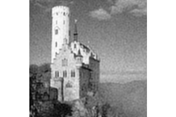
Writing this out is a bit of a pain, but it’s made a bit easier by noting that convolution with a 2D gaussian kernel is separable into two convolutions of 1D (e.g. convolve the image with the up-down filter, and do the same with the left-right) and by use of the Kronecker product to write out the individual matrices.⁴ The final $G$ is therefore the product of each of the convolutions. Just to show the comparison, here’s the initial image, taken from Wikipedia

Original greyscale image

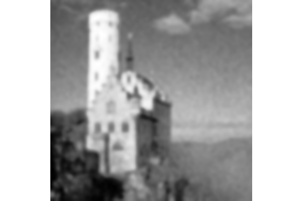
and here’s the image, blurred with a 2D gaussian kernel of size 5, with $\sigma =3$

Blurred greyscale image. The vignetting comes from edge effects.

The kernel, for context, looks like:

2D Gaussian Kernel with $N=5,\sigma =3$

Solving the problem, as given before, yields the final (almost identical) image:

The magical reconstructed image!

Which was nothing but solving a simple least squares problem (as we saw above)!

Now, you might say, “why are we going through all of this trouble to write this problem as a least-squares problem, when we can just take the FFT of the image and the gaussian and divide the former by the latter? Isn’t convolution just multiplication in the Fourier domain?”

And I would usually agree!

Except for one problem: while we may know the gaussian blurring operator on artificial images that we actively blur, the blurring operator that we provide for real images may not be fully representative of what’s really happening! By that I mean, if the real blurring operator is given by $G^{\text{real}}$, it could be that our guess $G$ is far away from $G^{\text{real}}$, perhaps because of some non-linear effects, or random noise, or whatever.

That is, we know what photos, in general, look like: they’re usually pretty smooth and have relatively few edges. In other words, the variations and displacements aren’t large almost everywhere in most images. This is where the multi-objective form of least-squares comes in handy—we can add a secondary (or third, etc) objective that allows us to specify how smooth the actual image should be!

How do we do this, you ask? Well, let’s consider the gradient at every point. If the gradient is large, then we’ve met an edge since there’s a large color variation between one pixel and its neighbour, similarly, if the gradient is small at that point, the image is relatively smooth at that point.

So, how about specifying that the sum of the norms of the gradients at every point be small?⁵ That is, we want the gradients to all be relatively small (minus those at edges, of course!), with some parameter that we can tune. In other words, let $D_x$ be the difference matrix between pixel $(i,j)$ and pixel $(i+1,j)$ (e.g. if our image is $X$ then $(D_{x}X{)}_{ij}=X_{i+1,j}-X_{ij}$, and, similarly, let $D_y$ be the difference matrix between pixel $(i,j)$ and $(i,j+1)$.⁶ Then our final objective is of the form

$$\underset{x}{\min }\Vert Gx-y{\Vert }^2+\lambda (\Vert D_{x}x{\Vert }^2+\Vert D_{y}x{\Vert }^2)$$

where $\lambda \ge 0$ is our ‘smoothness’ parameter. Note that, if we send $\lambda \to \infty$ then we really care that our image is ‘infinitely smooth’ (what would that look like?⁷), while if we send it to zero, we care that the reconstruction from the (possibly not great) approximation of $G^{\text{real}}$ is really good. Now, let’s compare the two methods with a slightly corrupted image:

The corrupted, blurred image we feed into the algorithm

Original greyscale image (again, for comparison)

Reconstruction with $\lambda ={10}^{-7}$

Reconstruction with original method

Though the normalized one has slightly larger grains, note that, unlike the original, the contrast isn’t as heavily lost and the edges, etc, are quite a bit sharper.

We can also toy a bit with the parameter, to get some intuition as to what all happens:

Reconstruction with $\lambda ={10}^{-3}$

Reconstruction with $\lambda ={10}^{-5}$

Reconstruction with $\lambda ={10}^{-10}$

Of course, as we make $\lambda$ large, note that the image becomes quite blurry (e.g. ‘smoother’), and as we send $\lambda$ to be very small, we end up with the same solution as the original problem, since we’re saying that we care very little about the smoothness and much more about the reconstruction approximation.

To that end, one could think of many more ways of characterizing a ‘natural’ image (say, if we know what some colors should look like, what is our usual contrast, etc.), all of which will yield successively better results, but I’ll leave with saying that LS, though relatively simple, is quite a powerful method for many cases. In particular, I’ll cover fully-constrained LS (in a more theoretical post) in the future, but with an application to path-planning.

Hopefully this was enough to convince you that even simple optimization methods are pretty useful! But if I didn’t do my job, maybe you’ll have to read some future posts. ;)

If you’d like, the complete code for this post can be found here.

In other words, that

$$f(y)\ge f(x^0),$$

for any $y$. But this is the definition of a global minimum since the point $f(x^0)$ is less than any other value the function takes on! So we’ve proved the claim that any local minimum (in fact, more strongly, that any point with vanishing derivative) is immediately a global minimum for a convex function. This is what makes convex functions so nice!

$$L=\left[\begin{array}{ccccc}1& -1& 0& 0& \dots \\ 0& 1& -1& 0& \dots \\ 0& 0& 1& -1& \dots \\ ⋮& ⋮& ⋮& ⋮& \ddots \end{array}\right]$$

this is relatively straightforward to form using an off-diagonal matrix. Note also that this matrix is quite sparse, which saves us from very large computation. Now, we want to apply this to each row (column) of the 2D image which is in row-major form. So, we follow the same idea as before and pre (post) multiply by the identity matrix. That is, for an $m\times m$ image

$$D_x=I_m\otimes L$$

and

$$D_y=L\otimes I_m$$

Footnotes

1. If $A^{T}Ax=0$ then $x^T{A}^{T}Ax=0$, but $x^T{A}^{T}Ax=(Ax{)}^T(Ax)=\Vert Ax{\Vert }^2=0$ which is zero only when $Ax=0$. E.g. only if there is an $x$ in the nullspace of $A$. ↩

2. A proof is straightforward. Let’s say $f$ is differentiable, since this is the case we care about, then we say $f$ is convex if the hyperplane given by $\nabla f(x)$ (at any $x$) bounds $f$ from below.

   A nice picture usually helps with this:

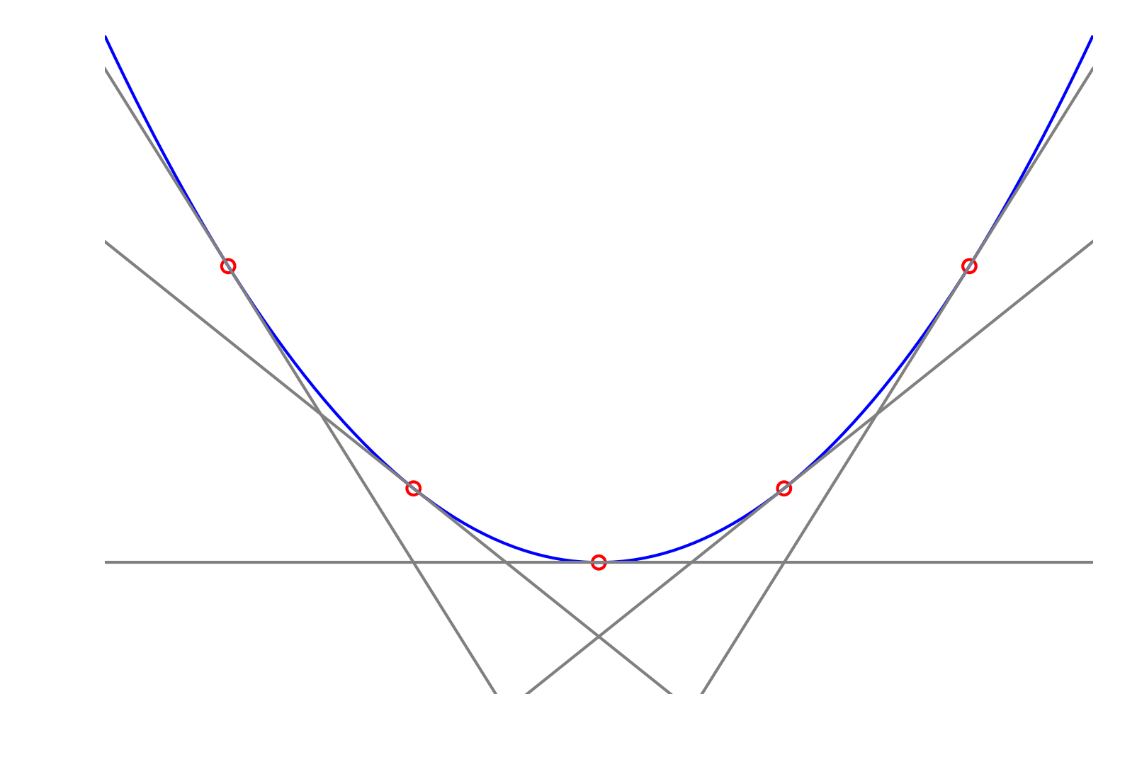
   Each of the hyperplanes (which are taken at the open, red circles along the curve; the hyperplanes themselves denoted by gray lines) always lies below the graph of the function (the blue parabola). We can write this as

   $$f(y)\ge (y-x{)}^T(\nabla f(x))+f(x)$$

   for all $x,y$.

   This is usually taken to be the definition of a convex function, so we’ll take it as such here. Now, if the point $x^0$ is a local minimum, we must have $\nabla f(x^0)=0$, this means that

   $$f(y)\ge (y-x^0{)}^T(\underset{=0}{\underbrace{\nabla f(x^0)}})+f(x^0)=(y-x^0{)}^{T}0+f(x^0)=f(x^0),$$

   for any $y$. ↩

3. There are, of course, better ways of doing this which I’ll present in some later post. For now, though, note that if the constraint is not achievable at equality, e.g. that we have $\Vert Cx-d{\Vert }^2\ge \epsilon >0$ for any $x$, then the objective ${\lambda }_i\Vert Cx-d{\Vert }^2\ge {\lambda }_i\epsilon \to \infty$ whenever we send ${\lambda }_i\to \infty$. This gives us a way of determining if the constraint is feasible (which happens only if the program converges to a finite value for arbitrarily increasing ${\lambda }_i$) or infeasible (which happens, as shown before, if the minimization program diverges to infinity). ↩

4. Assuming we write out the image as a row-major order, with dimensions $m\times m$, we can write the Toeplitz matrix of the 1D gaussian convolution of length $n$, say $T$. Then the row-convolution of the image’s one-dimensional vector representation is given by $I_m\otimes T$, where $\otimes$ denotes the Kronecker product of both matrices and $I_m$ is the $m\times m$ identity matrix. Similarly, we can do this for the column convolution by writing it out as $T\otimes I_{m+n}$ (note the additional $n$ which comes from the convolution!), then the final $G$ matrix is

   $$G=(T\otimes I_{m+n})(I_m\otimes T)$$

   which is much simpler to compute than the horrible initial expression dealing with indices. Additionally, these expressions are sparse (e.g. the first is block-diagonal), so we can exploit that to save on both memory and processing time. For more info, I’d recommend looking at the code for this entry. ↩

5. It turns out this has deep connections to a bunch of beautiful mathematical theories (most notably, the theory of heat diffusion on manifolds), but we won’t go into them here since it’s relatively out of scope, though I may cover it in a later post. ↩

6. These are slightly tricker to form for 2D images, but, as with the previous, we make heavy use of the Kronecker product. The derivative matrix for a 1D $m$-vector is the one formed by (let’s call it $L$ with dimensions $(m-1)\times m$) ↩

7. You probably guessed it: it’s just an image that is all the same color. ↩